% **Blog post code introduction**
%
% Congrats on activating the "All cells" option in this interactive blog post =D
%
% Below, several new HTML blocks have appears prior to the figures, displaying the Octave/MATLAB code that was used to generate the figures in this blog post.
%
% If you want to reproduce the data on your own local computer, you simply need to have qMRLab installed in your Octave/MATLAB path and run the "startup.m" file, as is shown below.
%
% If you want to get under the hood and modify the code right now, you can do so in the Jupyter Notebook of this blog post hosted on MyBinder. The link to it is in the introduction above.
Actual flip-angle imaging B1 mapping
Transmit radiofrequency field maps (B1+, or B1 for short) are used in diverse applications in MRI including: the study of electrical properties in tissues in vivo (Sled & Pike 1998; Katscher et al. 2009), specific absorption rate (SAR) calculations (Ibrahim et al. 2001), the calibration of quantitative T1 (Deoni 2007; Boudreau et al. 2017) and T2 (Sled and Pike 2000) maps, better parameter estimation from magnetization transfer measurements (Ropele et al. 2005; Boudreau et al. 2018), B1 shimming to improve image quality at whole-body ultra high fields (van den Bergen et al. 2007), or quality control of RF coils (Yarnykh 2007). Several B1 mapping techniques have been developed, and they can be broadly divided as magnitude-based and phase-based methods. The double angle method (DAM) is a saturation-recovery magnitude-based method that takes the ratio of the signal intensity of two magnitude images measured with different excitation flip angles (Insko & Bolinger 1993; Stollberger and Wach 1996). The Bloch-Siegert shift technique is a rapid phase-based method that encodes the B1 information into phase signal (Sacolick et al. 2010). The actual flip-angle imaging (AFI) is a magnitude-based B1 mapping method that consists of a 3D acquisition that benefits from good anatomical coverage. In addition, this technique allows the acquisitions of whole-body (~7 min) and brain (~3 min) B1 maps leading to a feasible implementation in clinics (Yarnykh 2004; Yarnykh 2007). On the other hand, the AFI pulse sequence has certain constraints that need to be considered for this B1 mapping method to be widely deployed. Some of the limitations include the use of spoiler gradients that can give rise to prohibitive SAR values (Sacolick et al. 2010), and the pulse sequence modifications on the MRI machine to implement the AFI method.
In this blog post, we will focus on presenting details about the AFI B1 mapping method. We will cover signal modeling, data fitting, the benefits and the pitfalls of the technique. The figures are generated using the qMRLab module for this method.
Signal Modelling
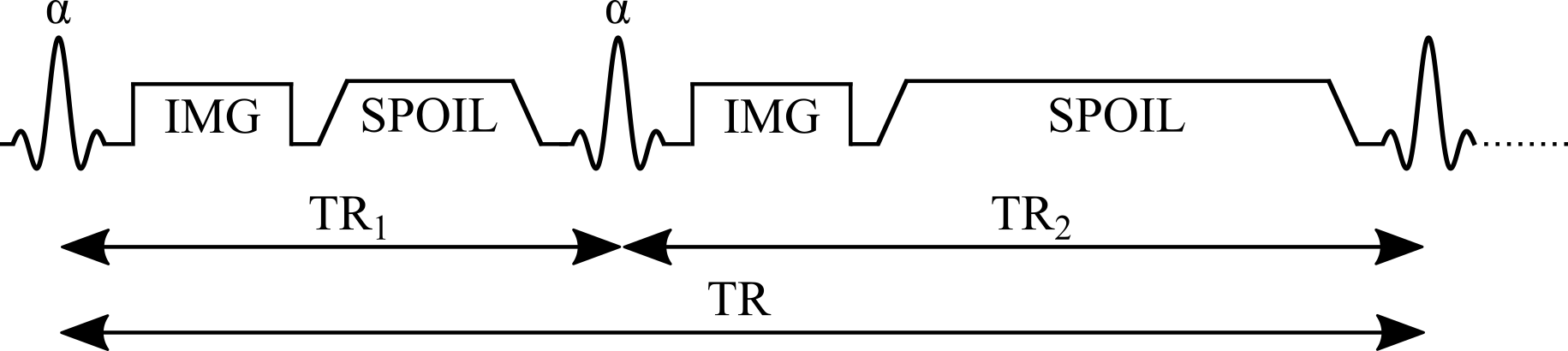
The pulse sequence of the AFI method (Figure 1) is composed of two identical RF pulses and two different delays (TR1 < TR2). After each RF pulse, the signal intensity is acquired followed by a spoiler to destroy the residual transverse magnetization next to the following RF pulse. This method implements a pulsed steady-state signal with a gradient-echo acquisition, thus preventing the use of long repetition times (Yarnykh 2007). It has been demonstrated that if the delays TR1 and TR2 are sufficiently short (e.g. TR1/TR2 = 20 ms/100 ms), and the transverse magnetization is completely spoiled, the ratio of signal intensities (r = S2/S1) depends on the flip angle of applied pulses and is highly insensitive to T1 (Yarnykh 2007).
Figure 1. Simplified pulse sequence diagram of an actual flip-angle imaging (AFI) pulse sequence with a gradient echo readout. TR1: repetition time 1, TR2: repetition time 2, θ: excitation flip angle for the measurement, IMG: image acquisition (k-space readout), SPOIL: spoiler gradient.
The magnetization of an AFI experiment can be modeled under steady-state conditions by the implementation of a fast repetition of the sequence (TR1 < TR2 < T1). The solution of the Bloch equations for the AFI method is given by Equations 1 and 2 that represent the longitudinal magnetization before the application of the RF pulses:


Mz1,2 is the longitudinal magnetization of both pulses, M0 is the magnetization at thermal equilibrium, TR1 is the delay time after the first pulse, TR2 is the delay time after the second identical pulse (Figure 1), and θ is the excitation flip angle. The steady-state longitudinal magnetization Mz curves for different T1 values for a range of θn and TR values are shown in Figure 2.
Figure 2. Longitudinal magnetization before the first radiofrequency pulse (Equation 1, solid lines) and before the second identical pulse (Equation 2, dashed lines) for three different T1 values.
%% MATLAB/OCTAVE CODE
% Adds qMRLab to the path of the environment

cd ../qMRLab
startup
%% MATLAB/OCTAVE CODE
% Code used to generate the data required for Figure 2 of the blog post

clear all

%% Setup parameters
% All times are in milliseconds
% All flip angles are in degrees

TR1_range = 5:5:50;
n = 5;
TR2_range = n*TR1_range;

params.EXC_FA = 1:90;

%% Calculate signals
%
% To see all the options available, run `help b1_afi.analytical_solution`

for ii = 1:length(TR1_range)
    params.TR1 = TR1_range(ii);
    params.TR2 = TR2_range(ii);

    % White matter
    params.T1 = 900; % in milliseconds
    [Mz1, Mz2] = b1_afi.analytical_solution(params);
    signal1_WM(ii,:) = Mz1;
    signal2_WM(ii,:) = Mz2;

    % Grey matter
    params.T1 = 1500;  % in milliseconds
    [Mz1, Mz2] = b1_afi.analytical_solution(params);
    signal1_GM(ii,:) = Mz1;
    signal2_GM(ii,:) = Mz2;

    % CSF
    params.T1 = 4000;  % in milliseconds
    [Mz1, Mz2] = b1_afi.analytical_solution(params);
    signal1_CSF(ii,:) = Mz1;
    signal2_CSF(ii,:) = Mz2;
end
# PYTHON CODE

init_notebook_mode(connected=True)

data1_1 = [dict(
        visible = False,
        line=dict(color='royalblue'),
        x = params["EXC_FA"],
        y = abs(np.squeeze(np.asarray(signal1_WM[ii]))),
        name = 'S<sub>1</sub>: T<sub>1</sub> = 0.9 s (White Matter)',
        text = 'S<sub>1</sub>: T<sub>1</sub> = 0.9 s (White Matter)',
        hoverinfo = 'x+y+text') for ii in range(len(TR1_range))]

data1_1[4]['visible'] = True

data1_2 = [dict(
        visible = False,
        line=dict(color='royalblue', dash='dash'),
        x = params["EXC_FA"],
        y = abs(np.squeeze(np.asarray(signal2_WM[ii]))),
        name = 'S<sub>2</sub>: T<sub>1</sub> = 0.9 s (White Matter)',
        text = 'S<sub>2</sub>: T<sub>1</sub> = 0.9 s (White Matter)',
        hoverinfo = 'x+y+text') for ii in range(len(TR1_range))]

data1_2[4]['visible'] = True

data2_1 = [dict(
        visible = False,
        line=dict(color='firebrick'),
        x = params["EXC_FA"],
        y = abs(np.squeeze(np.asarray(signal1_GM[ii]))),
        name = 'S<sub>1</sub>: T<sub>1</sub> = 1.5 s (Grey Matter)',
        text = 'S<sub>1</sub>: T<sub>1</sub> = 1.5 s (Grey Matter)',
        hoverinfo = 'x+y+text') for ii in range(len(TR1_range))]

data2_1[4]['visible'] = True

data2_2 = [dict(
        visible = False,
        line=dict(color='firebrick', dash='dash'),
        x = params["EXC_FA"],
        y = abs(np.squeeze(np.asarray(signal2_GM[ii]))),
        name = 'S<sub>2</sub>: T<sub>1</sub> = 1.5 s (Grey Matter)',
        text = 'S<sub>2</sub>: T<sub>1</sub> = 1.5 s (Grey Matter)',
        hoverinfo = 'x+y+text') for ii in range(len(TR1_range))]

data2_2[4]['visible'] = True

data3_1 = [dict(
        visible = False,
        line=dict(color='orange'),
        x = params["EXC_FA"],
        y = abs(np.squeeze(np.asarray(signal1_CSF[ii]))),
        name = 'S<sub>1</sub>: T<sub>1</sub> = 4.0 s (Cerebrospinal Fluid)',
        text = 'S<sub>1</sub>: T<sub>1</sub> = 4.0 s (Cerebrospinal Fluid)',
        hoverinfo = 'x+y+text') for ii in range(len(TR1_range))]

data3_1[4]['visible'] = True

data3_2 = [dict(
        visible = False,
        line=dict(color='orange', dash='dash'),
        x = params["EXC_FA"],
        y = abs(np.squeeze(np.asarray(signal2_CSF[ii]))),
        name = 'S<sub>2</sub>: T<sub>1</sub> = 4.0 s (Cerebrospinal Fluid)',
        text = 'S<sub>2</sub>: T<sub>1</sub> = 4.0 s (Cerebrospinal Fluid)',
        hoverinfo = 'x+y+text') for ii in range(len(TR1_range))]

data3_2[4]['visible'] = True

data = data1_1 + data1_2 + data2_1 +data2_2 + data3_1 + data3_2

steps = []
for i in range(len(TR1_range)):
    step = dict(
        method = 'restyle',
        args = ['visible', [False] * len(data1_1)],
        label = str(TR1_range[i])
        )
    step['args'][1][i] = True # Toggle i'th trace to "visible"
    steps.append(step)

sliders=[
    dict(
        x = 0,
        y = -0.09,
        active = 3,
        currentvalue = {"prefix": "TR1 value (ms): <b>"},
        pad = {"t": 50, "b": 10},
        steps = steps)]

layout = go.Layout(
    width=650,
    height=520,
    margin=go.layout.Margin(
        l=80,
        r=40,
        b=60,
        t=10,
    ),
    annotations=[
        dict(
            x=0.5004254919715793,
            y=-0.18,
            showarrow=False,
            text='Excitation Flip Angle (°)',
            font=dict(
                family='Times New Roman',
                size=22
            ),
            xref='paper',
            yref='paper'
        ),
        dict(
            x=-0.15,
            y=0.5,
            showarrow=False,
            text='Long. Magnetization (M<sub>z</sub>)',
            font=dict(
                family='Times New Roman',
                size=22
            ),
            textangle=-90,
            xref='paper',
            yref='paper'
        ),
        dict(
            x=-0.007,
            y=-0.25,
            showarrow=False,
            text='TR<sub>2</sub> = 5TR<sub>1</sub>',
            font=dict(
                family='Times New Roman',
                size=12
            ),
            xref='paper',
            yref='paper'
        ),
    ],
    xaxis=dict(
        autorange=False,
        range=[0, params['EXC_FA'][-1]],
        showgrid=False,
        linecolor='black',
        linewidth=2
    ),
    yaxis=dict(
        autorange=True,
        showgrid=False,
        linecolor='black',
        linewidth=2
    ),
    legend=dict(
        x=0.5,
        y=0.9,
        traceorder='normal',
        font=dict(
            family='Times New Roman',
            size=12,
            color='#000'
        ),
        bordercolor='#000000',
        borderwidth=2
    ),
    sliders=sliders
)

fig = dict(data=data, layout=layout)

iplot(fig, filename = 'basic-line', config = config)
The analytical solution of the Bloch equations in a steady-state experiment (Equation 1 and Equation 2) makes several assumptions leading to practical challenges. First, it is assumed that the longitudinal magnetization has reached a steady state after a sufficiently large number of repetition times (TR), and that the transverse magnetization is perfectly spoiled prior to each pulse. To explore these properties, a numerical approach known as Bloch simulations is used to estimate the signal from an MRI experiment given a set of sequence parameters. Here, the Bloch simulations allow us to estimate the magnetization using a different number of sequence repetitions, and look at a special case when the steady-state is not achieved (due to a small number of sequence repetitions). As can be seen in Figure 3, the number of repetitions required to reach a steady-state depends on T1 and the flip angle.
Figure 3. Signal 1 (blue) and Signal 2 (red) curves simulated using Bloch simulations (solid lines) for a number of repetitions ranging from 1 to 150, plotted against the ideal case (Equations 1 and 2 – dashed lines). Simulation details: TR1 = 20 ms, TR2 = 100 ms, T1 = 900 ms, 100 spins. Ideal spoiling was used for this set of Bloch simulations (transverse magnetization was set to 0 at the end of each TR1,2).
%% MATLAB/OCTAVE CODE
% Code used to generate the data required for Figure 3 of the blog post

clear all

%% Setup parameters
% All times are in milliseconds
% All flip angles are in degrees

% White matter
params.T1 = 900; % in milliseconds
params.T2 = 10000;
params.TR1 = 20;
params.TR2 = 100;
params.TE = 5;
params.EXC_FA = 1:90;
Nex_range = 1:1:150;

%% Calculate signals
% This results were precomputed. Uncomment the lines below to run the simulation.
signal1_bloch = load('../afi_blog/blochsim/signal1_blochsim.mat');
signal2_bloch = load('../afi_blog/blochsim/signal2_blochsim.mat');
signal1_analytical = load('../afi_blog/blochsim/signal1_analytical.mat');
signal2_analytical = load('../afi_blog/blochsim/signal2_analytical.mat');
signal1_blochsim = signal1_bloch.signal1_blochsim;
signal2_blochsim = signal2_bloch.signal2_blochsim;
signal1_analytical = signal1_analytical.signal1_analytical;
signal2_analytical = signal2_analytical.signal2_analytical;

%{
% Bloch simulations
% To see all the options available, run `help b1_afi.analytical_solution`

for ii = 1:length(Nex_range)
    params.Nex = Nex_range(ii);

    [Mz1, Mz2] = b1_afi.analytical_solution(params);
    signal1_analytical(ii,:) = Mz1;
    signal2_analytical(ii,:) = Mz2;

    [~, Msig1, Msig2] = b1_afi.bloch_sim(params);
    signal1_blochsim(ii,:) = abs(complex(Msig1));
    signal2_blochsim(ii,:) = abs(complex(Msig2));
end
%}
# PYTHON CODE

init_notebook_mode(connected=True)

data1_1 = [dict(
        visible = False,
        line=dict(color='royalblue', dash='dash'),
        x = params["EXC_FA"],
        y = abs(np.squeeze(np.asarray(signal1_analytical[ii]))),
        name = 'S<sub>1</sub>: Analytical Solution',
        text = 'S<sub>1</sub>: Analytical Solution',
        hoverinfo = 'x+y+text') for ii in range(len(Nex_range))]

data1_1[7]['visible'] = True

data1_2 = [dict(
        visible = False,
        line=dict(color='firebrick', dash='dash'),
        x = params["EXC_FA"],
        y = abs(np.squeeze(np.asarray(signal2_analytical[ii]))),
        name = 'S<sub>2</sub>: Analytical Solution',
        text = 'S<sub>2</sub>: Analytical Solution',
        hoverinfo = 'x+y+text') for ii in range(len(Nex_range))]

data1_2[7]['visible'] = True

data2_1 = [dict(
        visible = False,
        line=dict(color='royalblue'),
        x = params["EXC_FA"],
        y = abs(np.squeeze(np.asarray(signal1_blochsim[ii]))),
        name = 'S<sub>1</sub>: Bloch Simulation',
        text = 'S<sub>1</sub>: Bloch Simulation',
        hoverinfo = 'x+y+text') for ii in range(len(Nex_range))]

data2_1[7]['visible'] = True

data2_2 = [dict(
        visible = False,
        line=dict(color='firebrick'),
        x = params["EXC_FA"],
        y = abs(np.squeeze(np.asarray(signal2_blochsim[ii]))),
        name = 'S<sub>2</sub>: Bloch Simulation',
        text = 'S<sub>2</sub>: Bloch Simulation',
        hoverinfo = 'x+y+text') for ii in range(len(Nex_range))]

data2_2[7]['visible'] = True

data = data1_1 + data2_1 + data1_2 + data2_2

steps = []
for i in range(len(Nex_range)):
    step = dict(
        method = 'restyle',
        args = ['visible', [False] * len(data1_1)],
        label = str(Nex_range[i])
        )
    step['args'][1][i] = True # Toggle i'th trace to "visible"
    steps.append(step)

sliders = [dict(
    x = 0,
    y = -0.02,
    active = 5,
    currentvalue = {"prefix": "n<sup>th</sup> TR1-TR2: <b>"},
    pad = {"t": 50, "b": 10},
    steps = steps)]

layout = go.Layout(
    width=580,
    height=450,
    margin=go.layout.Margin(
        l=80,
        r=40,
        b=60,
        t=10,
    ),
    annotations=[
        dict(
            x=0.5004254919715793,
            y=-0.18,
            showarrow=False,
            text='Excitation Flip Angle (°)',
            font=dict(
                family='Times New Roman',
                size=22
            ),
            xref='paper',
            yref='paper'
        ),
        dict(
            x=-0.15,
            y=0.5,
            showarrow=False,
            text='Signal',
            font=dict(
                family='Times New Roman',
                size=22
            ),
            textangle=-90,
            xref='paper',
            yref='paper'
        ),
    ],
    xaxis=dict(
        autorange=False,
        range=[0, params['EXC_FA'][-1]],
        showgrid=False,
        linecolor='black',
        linewidth=2
    ),
    yaxis=dict(
        autorange=True,
        showgrid=False,
        linecolor='black',
        linewidth=2
    ),
    legend=dict(
        x=0.5,
        y=0.9,
        traceorder='normal',
        font=dict(
            family='Times New Roman',
            size=12,
            color='#000'
        ),
        bordercolor='#000000',
        borderwidth=2
    ),
    sliders=sliders
)

fig = dict(data=data, layout=layout)

iplot(fig, filename = 'basic-line', config = config)
In practice, gradient and RF spoiling are important parameters to consider in an AFI experiment. A combination of both (Zur et al. 1991; Bernstein et al. 2004) is typically recommended, and Figure 4 shows how this better approximates the ideal spoiling case.
Figure 4. Signal 1 curves estimated using Bloch simulations for three categories of signal spoiling: (1) ideal spoiling (blue), gradient & RF Spoiling (red), and no spoiling (orange). Simulation details: TR1 = 20 ms, TR2 = 100 ms, T1 = 900 ms, T2 = 100 ms, TE = 5 ms, 100 spins. For the ideal spoiling case, the transverse magnetization is set to zero at the end of each TR. For the gradient & RF spoiling case, each spin is rotated by different increments of phase (2𝜋 / # of spins) to simulate complete dephasing from gradient spoiling, and the RF phase of the excitation pulse is ɸn = ɸn-1 + nɸ0 = ½ ɸ0(n2 + n + 2) (Bernstein et al. 2004) with ɸ0 = 39° (Zur et al. 1991) after each TR.
%% MATLAB/OCTAVE CODE
% Code used to generate the data required for Figure 4 of the blog post

clear all

%% Setup parameters
% All times are in milliseconds
% All flip angles are in degrees

% White matter
params.T1 = 900; % in milliseconds
params.T2 = 100;
params.TR1 = 20;
params.TR2 = 100;
params.TE = 5;
params.EXC_FA = 1:90;
Nex_range = [1:9, 10:10:100];

%% Calculate signals
% This results were precomputed. Uncomment the lines below to run the simulation.
signal1_ideal = load('../afi_blog/blochsim/signal1_ideal_spoil.mat');
signal2_ideal = load('../afi_blog/blochsim/signal2_ideal_spoil.mat');
signal1_optimal = load('../afi_blog/blochsim/signal1_optimal_crush_and_rf_spoil.mat');
signal2_optimal = load('../afi_blog/blochsim/signal2_optimal_crush_and_rf_spoil.mat');
signal1_no_spoil = load('../afi_blog/blochsim/signal1_no_gradient_and_rf_spoil.mat');
signal2_no_spoil = load('../afi_blog/blochsim/signal2_no_gradient_and_rf_spoil.mat');
signal1_ideal_spoil = signal1_ideal.signal1_ideal_spoil;
signal2_ideal_spoil = signal2_ideal.signal2_ideal_spoil;
signal1_optimal_crush_and_rf_spoil = signal1_optimal.signal1_optimal_crush_and_rf_spoil;
signal2_optimal_crush_and_rf_spoil = signal2_optimal.signal2_optimal_crush_and_rf_spoil;
signal1_no_gradient_and_rf_spoil = signal1_no_spoil.signal1_no_gradient_and_rf_spoil;
signal2_no_gradient_and_rf_spoil = signal2_no_spoil.signal2_no_gradient_and_rf_spoil;

%{
% To see all the options available, run `help b1_afi.analytical_solution`

for ii = 1:length(Nex_range)
    params.Nex = Nex_range(ii);

    params.crushFlag = 1;

    [~, Msig1, Msig2] = b1_afi.bloch_sim(params);
    signal1_ideal_spoil(ii,:) = abs(Msig1);
    signal2_ideal_spoil(ii,:) = abs(Msig2);

    params.inc = 39;
    params.partialDephasing = 1;
    params.partialDephasingFlag = 1;
    params.crushFlag = 0;

    [~, Msig1, Msig2] = b1_afi.bloch_sim(params);
    signal1_optimal_crush_and_rf_spoil(ii,:) = abs(Msig1);
    signal2_optimal_crush_and_rf_spoil(ii,:) = abs(Msig2);

    params.inc = 0;
    params.partialDephasing = 0;

    [~, Msig1, Msig2] = b1_afi.bloch_sim(params);
    signal1_no_gradient_and_rf_spoil(ii,:) = abs(Msig1);
    signal2_no_gradient_and_rf_spoil(ii,:) = abs(Msig2);
end
%}
# PYTHON CODE

init_notebook_mode(connected=True)

data1_1 = [dict(
        visible = False,
        mode = 'lines',
        x = params["EXC_FA"],
        y = abs(np.squeeze(np.asarray(signal1_ideal_spoil[ii]))),
        name = 'Ideal Spoiling',
        text = 'Ideal Spoiling',
        hoverinfo = 'x+y+text') for ii in range(len(Nex_range))]

data1_1[10]['visible'] = True

data2_1 = [dict(
        visible = False,
        mode = 'lines',
        x = params["EXC_FA"],
        y = abs(np.squeeze(np.asarray(signal1_optimal_crush_and_rf_spoil[ii]))),
        name = 'Gradient & RF Spoiling',
        text = 'Gradient & RF Spoiling',
        hoverinfo = 'x+y+text') for ii in range(len(Nex_range))]

data2_1[10]['visible'] = True

data3_1 = [dict(
        visible = False,
        mode = 'lines',
        x = params["EXC_FA"],
        y = abs(np.squeeze(np.asarray(signal1_no_gradient_and_rf_spoil[ii]))),
        name = 'No Spoiling',
        text = 'No Spoiling',
        hoverinfo = 'x+y+text') for ii in range(len(Nex_range))]

data3_1[10]['visible'] = True

data = data1_1 + data2_1+ data3_1

steps = []
for i in range(len(Nex_range)):
    step = dict(
        method = 'restyle',
        args = ['visible', [False] * len(data1_1)],
        label = str(Nex_range[i])
        )
    step['args'][1][i] = True # Toggle i'th trace to "visible"
    steps.append(step)

sliders = [dict(
    x = 0,
    y = -0.02,
    active = 10,
    currentvalue = {"prefix": "n<sup>th</sup> TR1-TR2: <b>"},
    pad = {"t": 50, "b": 10},
    steps = steps
)]

layout = go.Layout(
    width=580,
    height=450,
    margin=go.layout.Margin(
        l=80,
        r=40,
        b=60,
        t=10,
    ),
    annotations=[
        dict(
            x=0.5004254919715793,
            y=-0.18,
            showarrow=False,
            text='Excitation Flip Angle (°)',
            font=dict(
                family='Times New Roman',
                size=22
            ),
            xref='paper',
            yref='paper'
        ),
        dict(
            x=-0.15,
            y=0.5,
            showarrow=False,
            text='Signal',
            font=dict(
                family='Times New Roman',
                size=22
            ),
            textangle=-90,
            xref='paper',
            yref='paper'
        ),
    ],
    xaxis=dict(
        autorange=False,
        range=[0, params['EXC_FA'][-1]],
        showgrid=False,
        linecolor='black',
        linewidth=2
    ),
    yaxis=dict(
        autorange=True,
        showgrid=False,
        linecolor='black',
        linewidth=2
    ),
    legend=dict(
        x=0.5,
        y=0.9,
        traceorder='normal',
        font=dict(
            family='Times New Roman',
            size=12,
            color='#000'
        ),
        bordercolor='#000000',
        borderwidth=2
    ),
    sliders=sliders
)

fig = dict(data=data, layout=layout)

iplot(fig, filename = 'basic-line', config = config)
Data Fitting
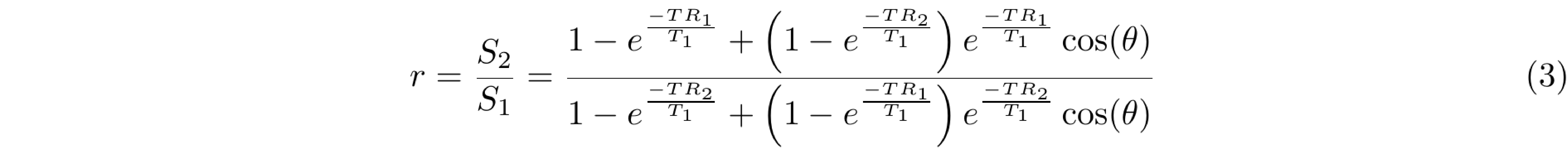
The ratio of Equations 1 and 2, gives rise to Equation 3 that depends on the parameters T1, TR1, TR2 and the excitation flip angle (θ).
Equation 3 can be simplified if the Taylor series expansion of the exponential function is used, followed by a first-order approximation to its terms. For this expansion, short TR1 and TR2 (TR1 < T1 and TR2 < T1) are assumed to approximate the signal intensities ratio (Equation 4) where n = TR2/TR1.

Finally, a measure of the actual flip-angle (θ) can be achieved by solving Equation 4 to obtain Equation 5, which only depends on the signal intensities ratio (r = S2/S1) and the parameters TR1 and TR2.

The actual flip-angle is estimated using an approximation (Equation 4) of a complete analytical solution (Equation 3), and the nature of this approximation makes it worthwhile to assess the accuracy of the signal intensities ratio between both equations. Next, a set of simulations are displayed to analyze how the choice of r is affected by T1, TR1 and TR2. First, the effect of the relaxation time T1 is simulated in Figure 5 for both the approximation and the complete analytical solution.
Figure 5. Effect of the relaxation time T1 on the ratio r. Signal intensities ratio is plotted as a function of the flip angle for the complete analytical solution (Equation 3 - blue) and the first-order approximation (Equation 4 - orange). AFI simulation details: TR1 = 20 ms, TR2 = 100 ms and variable T1.
%% MATLAB/OCTAVE CODE
% Code used to generate the data required for Figure 5 of the blog post

clear all

%% Setup parameters
% All times are in milliseconds
% All flip angles are in degrees

%% Calculate signals
%
% To see all the options available, run `help b1_afi.analytical_solution`

T1_range = [10:10:200, 200:400:2000];

params.TR1 = 20;
params.TR2 = 100;
params.EXC_FA = 1:90;
n = params.TR2/params.TR1;

for jj=1:length(T1_range)
    params.T1 = T1_range(jj);

    % Range of T1
    [Mz1, Mz2] = b1_afi.analytical_solution(params);
    signal1_analytical = Mz1;
    signal2_analytical = Mz2;

    r_analytical(jj,:) = signal2_analytical./signal1_analytical;
    r_approximation(jj,:) = (1 + n.*cosd(params.EXC_FA))./(n + cosd(params.EXC_FA));
end
# PYTHON CODE

init_notebook_mode(connected=True)

data1 = [dict(
        visible = False,
        mode = 'lines',
        x = params["EXC_FA"],
        y = abs(np.squeeze(np.asarray(r_analytical[ii]))),
        name = 'Analytical',
        text = 'Analytical',
        hoverinfo = 'x+y+text') for ii in range(len(T1_range))]

data1[10]['visible'] = True

data2 = [dict(
        visible = False,
        mode = 'lines',
        x = params["EXC_FA"],
        y = abs(np.squeeze(np.asarray(r_approximation[ii]))),
        name = 'Approximation',
        text = 'Approximation',
        hoverinfo = 'x+y+text') for ii in range(len(T1_range))]

data2[10]['visible'] = True

data = data1 + data2

steps = []
for i in range(len(T1_range)):
    step = dict(
        method = 'restyle',
        args = ['visible', [False] * len(data1)],
        label = str(T1_range[i])
        )
    step['args'][1][i] = True # Toggle i'th trace to "visible"
    steps.append(step)

sliders = [dict(
    x = 0,
    y = -0.02,
    active = 10,
    currentvalue = {"prefix": "T1 value (ms): <b>"},
    pad = {"t": 50, "b": 10},
    steps = steps)]

layout = go.Layout(
    width=580,
    height=450,
    margin=go.layout.Margin(
        l=80,
        r=40,
        b=60,
        t=10,
    ),
    annotations=[
        dict(
            x=0.5004254919715793,
            y=-0.18,
            showarrow=False,
            text='Excitation Flip Angle (°)',
            font=dict(
                family='Times New Roman',
                size=22
            ),
            xref='paper',
            yref='paper'
        ),
        dict(
            x=-0.15,
            y=0.5,
            showarrow=False,
            text='r = S<sub>2</sub>/S<sub>1</sub>',
            font=dict(
                family='Times New Roman',
                size=22
            ),
            textangle=-90,
            xref='paper',
            yref='paper'
        ),
    ],
    xaxis=dict(
        autorange=False,
        range=[0, params['EXC_FA'][-1]],
        showgrid=False,
        linecolor='black',
        linewidth=2
    ),
    yaxis=dict(
        autorange=True,
        showgrid=False,
        linecolor='black',
        linewidth=2
    ),
    legend=dict(
        x=0.5,
        y=0.9,
        traceorder='normal',
        font=dict(
            family='Times New Roman',
            size=12,
            color='#000'
        ),
        bordercolor='#000000',
        borderwidth=2
    ),
    sliders=sliders
)

fig = dict(data=data, layout=layout)

iplot(fig, filename = 'basic-line', config = config)
The signal ratio r is highly insensitive to the relaxation time T1, except for the low T1 values and large flip angles (>70°). This shows that the Taylor expansion is a good approximation to the signal ratio r because it is possible to get rid of the inverse quadratic T1 dependance by taking the first-order terms of the expansion.
The effect of the TR1 parameter on the signal ratio is shown in Figure 6. To assess the influence of the repetition time, we fix n=5 and vary the parameter TR1 in accordance to the relation n = TR2/TR1. As TR1 increases (> 50 ms), the approximated ratio r slightly deviates from the analytical approach. Although the deviation is slight only at high flip angles, a good signal ratio approximation can be achieved for a wide range of flip angles and repetition times.
Figure 6. Effect of the repetition time TR1 on the ratio r. Signal intensities ratio is plotted as a function of the flip angle for the complete analytical solution (Equation 3 - blue) and the first-order approximation (Equation 4 - orange). AFI simulation details: Variable TR1 ranging from 10 to 60 ms, fixed ratio n = 5 and T1 = 900 ms.
%% MATLAB/OCTAVE CODE
% Code used to generate the data required for Figure 6 of the blog post

clear all

%% Setup parameters
% All times are in milliseconds
% All flip angles are in degrees

%% Calculate signals
%
% To see all the options available, run `help b1_afi.analytical_solution`

TR1_range = 10:5:60;

params.T1 = 900;
params.EXC_FA = 1:90;
n = 5;

for jj=1:length(TR1_range)
    params.TR1 = TR1_range(jj);
    params.TR2 = n*params.TR1;

    % Fixed: T1 = 900 ms, n = 5
    [Mz1, Mz2] = b1_afi.analytical_solution(params);
    signal1_analytical = Mz1;
    signal2_analytical = Mz2;

    r_analytical(jj,:) = signal2_analytical./signal1_analytical;
    r_approximation(jj,:) = (1 + n.*cosd(params.EXC_FA))./(n + cosd(params.EXC_FA));
end
# PYTHON CODE

init_notebook_mode(connected=True)

data1 = [dict(
        visible = False,
        mode = 'lines',
        x = params["EXC_FA"],
        y = abs(np.squeeze(np.asarray(r_analytical[ii]))),
        name = 'Analytical',
        text = 'Analytical',
        hoverinfo = 'x+y+text') for ii in range(len(TR1_range))]

data1[2]['visible'] = True

data2 = [dict(
        visible = False,
        mode = 'lines',
        x = params["EXC_FA"],
        y = abs(np.squeeze(np.asarray(r_approximation[ii]))),
        name = 'Approximation',
        text = 'Approximation',
        hoverinfo = 'x+y+text') for ii in range(len(TR1_range))]

data2[2]['visible'] = True

data = data1 + data2

steps = []
for i in range(len(TR1_range)):
    step = dict(
        method = 'restyle',
        args = ['visible', [False] * len(data1)],
        label = str(TR1_range[i])
        )
    step['args'][1][i] = True # Toggle i'th trace to "visible"
    steps.append(step)

sliders = [dict(
    x = 0,
    y = -0.02,
    active = 2,
    currentvalue = {"prefix": "TR1 value (ms): <b>"},
    pad = {"t": 50, "b": 10},
    steps = steps)]

layout = go.Layout(
    width=580,
    height=450,
    margin=go.layout.Margin(
        l=80,
        r=40,
        b=60,
        t=10,
    ),
    annotations=[
        dict(
            x=0.5004254919715793,
            y=-0.18,
            showarrow=False,
            text='Excitation Flip Angle (°)',
            font=dict(
                family='Times New Roman',
                size=22
            ),
            xref='paper',
            yref='paper'
        ),
        dict(
            x=-0.15,
            y=0.5,
            showarrow=False,
            text='r = S<sub>2</sub>/S<sub>1</sub>',
            font=dict(
                family='Times New Roman',
                size=22
            ),
            textangle=-90,
            xref='paper',
            yref='paper'
        ),
    ],
    xaxis=dict(
        autorange=False,
        range=[0, params['EXC_FA'][-1]],
        showgrid=False,
        linecolor='black',
        linewidth=2
    ),
    yaxis=dict(
        autorange=True,
        showgrid=False,
        linecolor='black',
        linewidth=2
    ),
    legend=dict(
        x=0.5,
        y=0.9,
        traceorder='normal',
        font=dict(
            family='Times New Roman',
            size=12,
            color='#000'
        ),
        bordercolor='#000000',
        borderwidth=2
    ),
    sliders=sliders
)

fig = dict(data=data, layout=layout)

iplot(fig, filename = 'basic-line', config = config)
Finally, the effect of the parameter n on the signal ratio r (Figure 7) does not seem to significantly affect the signal ratio between the approximated equation and the analytical approach. However, the parameter n has a major impact on the sensitivity of the AFI method to variations in the flip angle. Figure 7 shows that the increase of the parameter n (= TR2/TR1) allows for improvement of the dynamic range of flip angles measurements. These simulations have shown that an optimal implementation of the AFI method requires a careful selection of sequence parameters.
Figure 7. Effect of n (TR2 to TR1 ratio) on the ratio r. The signal intensities ratio is plotted as a function of the flip angle for the complete analytical solution (Equation 3 - blue) and the first-order approximation (Equation 4 - orange). AFI simulation details: Variable n ranging from 2 to 6, fixed TR1 = 20 ms and T1 = 900 ms.
%% MATLAB/OCTAVE CODE
% Code used to generate the data required for Figure 7 of the blog post

clear all

%% Setup parameters
% All times are in milliseconds
% All flip angles are in degrees

%% Calculate signals
%
% To see all the options available, run `help b1_afi.analytical_solution`

n_range = 2:1:6;

params.T1 = 900;
params.TR1 = 20;
params.EXC_FA = 1:90;

for jj=1:length(n_range)
    n = n_range(jj);
    params.TR2 = n*params.TR1;

    % Fixed: T1 = 900 ms, TR1 = 20
    [Mz1, Mz2] = b1_afi.analytical_solution(params);
    signal1_analytical = Mz1;
    signal2_analytical = Mz2;

    r_analytical(jj,:) = signal2_analytical./signal1_analytical;
    r_approximation(jj,:) = (1 + n.*cosd(params.EXC_FA))./(n + cosd(params.EXC_FA));
end
# PYTHON CODE

init_notebook_mode(connected=True)

data1 = [dict(
        visible = False,
        mode = 'lines',
        x = params["EXC_FA"],
        y = abs(np.squeeze(np.asarray(r_analytical[ii]))),
        name = 'Analytical',
        text = 'Analytical',
        hoverinfo = 'x+y+text') for ii in range(len(n_range))]

data1[2]['visible'] = True

data2 = [dict(
        visible = False,
        mode = 'lines',
        x = params["EXC_FA"],
        y = abs(np.squeeze(np.asarray(r_approximation[ii]))),
        name = 'Approximation',
        text = 'Approximation',
        hoverinfo = 'x+y+text') for ii in range(len(n_range))]

data2[2]['visible'] = True

data = data1 + data2

steps = []
for i in range(len(n_range)):
    step = dict(
        method = 'restyle',
        args = ['visible', [False] * len(data1)],
        label = str(n_range[i])
        )
    step['args'][1][i] = True # Toggle i'th trace to "visible"
    steps.append(step)

sliders = [dict(
    x = 0,
    y = -0.02,
    active = 2,
    currentvalue = {"prefix": "n value: <b>"},
    pad = {"t": 50, "b": 10},
    steps = steps)]

layout = go.Layout(
    width=580,
    height=450,
    margin=go.layout.Margin(
        l=80,
        r=40,
        b=60,
        t=10,
    ),
    annotations=[
        dict(
            x=0.5004254919715793,
            y=-0.18,
            showarrow=False,
            text='Excitation Flip Angle (°)',
            font=dict(
                family='Times New Roman',
                size=22
            ),
            xref='paper',
            yref='paper'
        ),
        dict(
            x=-0.15,
            y=0.5,
            showarrow=False,
            text='r = S<sub>2</sub>/S<sub>1</sub>',
            font=dict(
                family='Times New Roman',
                size=22
            ),
            textangle=-90,
            xref='paper',
            yref='paper'
        ),
    ],
    xaxis=dict(
        autorange=False,
        range=[0, params['EXC_FA'][-1]],
        showgrid=False,
        linecolor='black',
        linewidth=2
    ),
    yaxis=dict(
        autorange=False,
        range=[0, 1],
        showgrid=False,
        linecolor='black',
        linewidth=2
    ),
    legend=dict(
        x=0.5,
        y=0.9,
        traceorder='normal',
        font=dict(
            family='Times New Roman',
            size=12,
            color='#000'
        ),
        bordercolor='#000000',
        borderwidth=2
    ),
    sliders=sliders
)

fig = dict(data=data, layout=layout)

iplot(fig, filename = 'basic-line', config = config)
Figure 8 displays an example AFI dataset and its corresponding field B1 map in a healthy human brain. Although not clearly visible, both AFI images present a small Gibbs ringing artifact that is propagated and amplified due to the AFI calculation consisting of the division of both images (Boudreau et al. 2017). The ringing artifact is clearly seen in the unfiltered/raw B1 field map shown in Figure 8 (right).
Figure 8. Example actual flip-angle imaging dataset (left) and a resulting raw B1 map of a healthy adult brain (right). The relevant VFA protocol parameters used were: TR1 = 20 ms, TR2 = 100 ms and θnominal = 60°. The B1 map (right) was fitted using the approximate r ratio (Equation 5).
%% MATLAB/OCTAVE CODE
% Download Actual Flip-Angle Imaging brain MRI data for Figure 8 of the blog post

cmd = ['curl -L -o b1_afi.zip https://osf.io/csjgx/download?version=6'];
[STATUS,MESSAGE] = unix(cmd);
unzip('b1_afi.zip');
%% MATLAB/OCTAVE CODE
% Code used to generate the data required for Figure 8 of the blog post

clear all

% Format qMRLab b1_afi model parameters, and load them into the Model object
Model = b1_afi;
Model.Prot.Sequence.Mat = [60, 20, 100];

% Format data structure so that they may be fit by the model
data = struct();
data.AFIData1 = load_nii_data('b1_afi/AFIData1.nii.gz');
data.AFIData2 = load_nii_data('b1_afi/AFIData2.nii.gz');

FitResults = FitData(data,Model,0); % The '0' flag is so that no wait bar is shown.
%% MATLAB/OCTAVE CODE
% Code used to re-orient the images to make pretty figures, and to assign variables with the axis lengths.

B1map_raw = imrotate(squeeze(FitResults.B1map_raw(:,:,14)),-90);

xAxis = [0:size(B1map_raw,2)-1];
yAxis = [0:size(B1map_raw,1)-1];

% Raw MRI AFI data
AFIData1 = imrotate(squeeze(data.AFIData1(:,:,14)),-90);
AFIData2 = imrotate(squeeze(data.AFIData2(:,:,14)),-90);

% Load mask
mask = load_nii_data('../afi_blog/fitResults/FitResults_median_filter/mask.nii.gz');
mask = imrotate(squeeze(mask(:,:,14)),-90);
from plotly import tools

# Masking B1 map
B1map_raw = np.asarray(B1map_raw)
mask = np.asarray(mask)
B1map_raw_masked = B1map_raw*mask
B1map_raw_masked[np.isnan(B1map_raw_masked)] = 0


trace1 = go.Heatmap(x = xAxis,
                   y = yAxis,
                   z=AFIData1,
                   colorscale='Greys',
                   showscale = False,
                   visible=False,
                   name = 'Signal1')
trace2 = go.Heatmap(x = xAxis,
                   y = yAxis,
                   z=AFIData2,
                   colorscale='Greys',
                   showscale = False,
                   visible=True,
                   name = 'Signal2')
trace3 = go.Heatmap(x = xAxis,
                   y = yAxis,
                   z=B1map_raw_masked,
                   zmin=0.7,
                   zmax=1.3,
                   colorscale='RdBu',
                   xaxis='x2',
                   yaxis='y2',
                   visible=True,
                   name = 'B1 values')

data=[trace1, trace2, trace3]


updatemenus = list([
    dict(active=1,
         x = 0.09,
         xanchor = 'left',
         y = -0.15,
         yanchor = 'bottom',
         direction = 'up',
         font=dict(
                family='Times New Roman',
                size=16
            ),
         buttons=list([
            dict(label = 'Signal 1',
                 method = 'update',
                 args = [{'visible': [True, False, True]},
                         ]),
            dict(label = 'Signal 2',
                 method = 'update',
                 args = [{'visible': [False, True, True]},
                           ]),
        ])
    )
])

layout = dict(
    width=560,
    height=345,
    margin = dict(
                t=40,
                r=50,
                b=10,
                l=50),
    annotations=[
        dict(
            x=0.07,
            y=1.15,
            showarrow=False,
            text='Input Data',
            font=dict(
                family='Times New Roman',
                size=26
            ),
            xref='paper',
            yref='paper'
        ),
        dict(
            x=0.60,
            y=1.15,
            showarrow=False,
            text='Raw B<sub>1</sub> map',
            font=dict(
                family='Times New Roman',
                size=26
            ),
            xref='paper',
            yref='paper'
        ),
        dict(
            x=1.12,
            y=1.15,
            showarrow=False,
            text='B<sub>1</sub>',
            font=dict(
                family='Times New Roman',
                size=26
            ),
            xref='paper',
            yref='paper'
        ),
    ],
    xaxis = dict(range = [0,127], autorange = False,
             showgrid = False, zeroline = False, showticklabels = False,
             ticks = '', domain=[0, 0.58]),
    yaxis = dict(range = [0,127], autorange = False,
             showgrid = False, zeroline = False, showticklabels = False,
             ticks = '', domain=[0, 1]),
    xaxis2 = dict(range = [0,127], autorange = False,
             showgrid = False, zeroline = False, showticklabels = False,
             ticks = '', domain=[0.40, 0.98]),
    yaxis2 = dict(range = [0,127], autorange = False,
             showgrid = False, zeroline = False, showticklabels = False,
             ticks = '', domain=[0, 1], anchor='x2'),
    showlegend = False,
    autosize = False,
    updatemenus=updatemenus
)


fig = dict(data=data, layout=layout)

iplot(fig, filename = 'basic-heatmap', config = config)
The ringing artifact shown in Figure 8 can be attenuated by implementing a smoothing process. Figure 9 shows the raw (left) and the filtered (right) B1 map where a median filter was used to smooth the field map.
Figure 9. Raw (left) and filtered (right) B1 map. A median filter of size 7x7x7 pixels was used to attenuate the Gibbs ringing artifact.
B1map_filtered = load_nii_data('../afi_blog/fitResults/FitResults_median_filter/B1map_filtered.nii.gz');
B1map_filtered = imrotate(squeeze(B1map_filtered(:,:,14)),-90);
from plotly import tools

# Masking B1 map
B1map_filtered = np.asarray(B1map_filtered)
mask = np.asarray(mask)
B1map_filtered_masked = B1map_filtered*mask
B1map_filtered_masked[np.isnan(B1map_filtered_masked)] = 0

trace1 = go.Heatmap(x = xAxis,
                   y = yAxis,
                   z=B1map_raw_masked,
                   zmin=0.7,
                   zmax=1.3,
                   colorscale='RdBu',
                   showscale = False,
                   visible=True,
                   name = 'B1 values')
trace2 = go.Heatmap(x = xAxis,
                   y = yAxis,
                   z=B1map_filtered_masked,
                   zmin=0.7,
                   zmax=1.3,
                   colorscale='RdBu',
                   xaxis='x2',
                   yaxis='y2',
                   visible=True,
                   name = 'B1 values')

data=[trace1, trace2]

layout = dict(
    width=560,
    height=310,
    margin = dict(
                t=40,
                r=50,
                b=10,
                l=50),
    annotations=[
        dict(
            x=0.04,
            y=1.15,
            showarrow=False,
            text='Raw B<sub>1</sub> map',
            font=dict(
                family='Times New Roman',
                size=26
            ),
            xref='paper',
            yref='paper'
        ),
        dict(
            x=0.60,
            y=1.15,
            showarrow=False,
            text='Filtered B<sub>1</sub> map',
            font=dict(
                family='Times New Roman',
                size=26
            ),
            xref='paper',
            yref='paper'
        ),
        dict(
            x=1.12,
            y=1.15,
            showarrow=False,
            text='B<sub>1</sub>',
            font=dict(
                family='Times New Roman',
                size=26
            ),
            xref='paper',
            yref='paper'
        ),
    ],
    xaxis = dict(range = [0,127], autorange = False,
             showgrid = False, zeroline = False, showticklabels = False,
             ticks = '', domain=[0, 0.58]),
    yaxis = dict(range = [0,127], autorange = False,
             showgrid = False, zeroline = False, showticklabels = False,
             ticks = '', domain=[0, 1]),
    xaxis2 = dict(range = [0,127], autorange = False,
             showgrid = False, zeroline = False, showticklabels = False,
             ticks = '', domain=[0.40, 0.98]),
    yaxis2 = dict(range = [0,127], autorange = False,
             showgrid = False, zeroline = False, showticklabels = False,
             ticks = '', domain=[0, 1], anchor='x2'),
    showlegend = False,
    autosize = False,
)


fig = dict(data=data, layout=layout)

iplot(fig, filename = 'basic-heatmap', config = config)
Benefits and Pitfalls
B1 mapping is of interest for diverse MRI applications, and several mapping techniques have been developed. The DAM method consists of acquiring two scans at two different flip angles. To avoid the dependence of the signal on T1, long repetition times are required to allow the recovery of the longitudinal magnetization between pulses (Yarnykh 2007; Insko & Bolinger 1993). The AFI method overcomes this practical limitation by repeating the pulse sequence at a fast rate to achieve a pulsed state of magnetization and shorter time delays between pulses. In addition, due to scan-time constraints, B1 mapping methods are often implemented in 2D (Chavez & Stanisz 2011). However, the accuracy of the measurements of 2D B1 mapping techniques is compromised by the slice profile effects due to the problem of nonuniform excitation across slices (Yarnykh 2007; Chavez & Stanisz 2011). The AFI method on the other hand, adresses this issue using a fast 3D implementation leading to scans with an excellent anatomical coverage in clinically feasible times, with an increase in signal-to-noise ratio compared to 2D multislice acquisitions.
The performance of the AFI method is based on the following assumptions. First, the two images acquired at different times should be registered to avoid motion effects. It is also assumed that the signal is insensitive to the main magnetic field non-uniformities and chemical shift effects that are canceled out when taking the signal ratio r (Yarnykh 2007). Despite some clear advantages over other B1 mapping techniques, the application of spoiler gradients to mitigate the T1 dependence can be a limitation due to significant levels of RF power depositions (Sacolick et al. 2010). Furthermore, it is necessary to adapt the AFI pulse sequence to different scanner manufacturers, and programming experience is required to bring this technique into the clinic.
Works Cited
Bernstein, M., King, K. & Zhou, X., 2004. Handbook of MRI Pulse Sequences, Elsevier.
Boudreau, M., Tardif, C.L., Stikov, N., Sled, J.G., Lee, W. & Pike, G.B., 2017. B1 mapping for bias-correction in quantitative T1 imaging of the brain at 3T using standard pulse sequences. J. Magn. Reson. Imaging, 46, pp.1673-1682.
Boudreau, M., Stikov, N. & Pike, G.B, 2018. B1-sensitivity analysis of quantitative magnetization transfer imaging. Magn. Reson. Med., 79, pp.276-285.
Chavez, S. & Stanisz, G.J., 2012. A novel method for simultaneous 3D B1 and T1 mapping: the method of slopes (MoS). NMR Biomed., 25, pp.1043-1055.
Deoni, S.C., 2007. High-resolution T1 mapping of the brain at 3T with driven equilibrium single pulse observation of T1 with high-speed incorporation of RF field inhomogeneities (DESPOT1-HIFI). J. Magn. Reson. Imaging, 26, pp.1106-1111.
Ibrahim, T.S., Lee, R., Baertlein, B.A. & Robitaille, P.M., 2001. B1 field homogeneity and SAR calculations for the birdcage coil. Phys Med Biol., 46(2), pp.609-619.
Insko, E. & Bolinger, L., 1993. Mapping of the radio frequency field. J. Magn. Reson. Ser. A, 103(1), pp.82–85.
Katscher, U., Voigt, T., Findeklee, C., Vernickel, P., Nehrke, K. & Dössel, O., 2009. Determination of electric conductivity and local SAR via B1 mapping. IEEE Trans Med Imaging., 28(9), pp.1365-1374.
Ropele, S., Filippi, M., Valsasina, P., Korteweg, T., Barkhof, F., Tofts, P.S., Samson, R., Miller, D.H. & Fazekas, F., 2005. Assessment and correction of B1-induced errors in magnetization transfer ratio measurements. Magn. Reson. Med., 53, pp.134-140.
Sacolick, L.I., Wiesinger, F., Hancu, I. & Vogel, M.W., 2010. B1 mapping by Bloch-Siegert shift. Magn. Reson. Med., 63, pp.1315-1322.
Sled, J.G. & Pike, G.B., 1998. Standing-wave and RF penetration artifacts caused by elliptic geometry: an electrodynamic analysis of MRI. IEEE Trans. Med. Imaging., 17(4), pp.653-662.
Sled, J.G. & Pike, G.B., 2000. Correction for B1 and B0 variations in quantitative T2 measurements using MRI. Magn. Reson. Med., 43(4), pp.589–593.
Stollberger, R. & Wach, P., 1996. Imaging of the active B1 field in vivo. Magn. Reson. Med., 35(2), pp.246–251.
van den Bergen, B., Van den Berg, C.A., Bartels, L.W. & Lagendijk, J.J., 2007. 7 T body MRI: B1 shimming with simultaneous SAR reduction. Phys Med Biol., 52(17), pp.5429-5441.
Yarnykh, V.L. & Yuan, C. Actual flip angle imaging in the pulsed steady state. In: Proceedings of the 12th Annual Meeting of ISMRM, Kyoto, Japan, 2004 (Abstract 194).
Yarnykh, V.L., 2007. Actual Flip-Angle Imaging in the pulsed steady state: A method for rapid three-dimensional mapping of the transmitted radiofrequency field. Magn. Reson. Med., 57(1), pp.192-200.
Yarnykh, V.L., 2010. Optimal radiofrequency and gradient spoiling for improved accuracy of T1 and B1 measurements using fast steady-state techniques. Magn. Reson. Med., 63(6), pp.1610–1626.
Zur, Y., Wood, M.L. & Neuringer, L.J., 1991. Spoiling of transverse magnetization in steady-state sequences. Magn. Reson. Med., 21(2), pp.251–263.
# PYTHON CODE

display(HTML(
    '<style type="text/css">'
    '.output_subarea {'
        'display: block;'
        'margin-left: auto;'
        'margin-right: auto;'
    '}'
    '.blog_body {'
        'line-height: 2;'
        'font-family: timesnewroman;'
        'font-size: 18px;'
        'margin-left: 0px;'
        'margin-right: 0px;'
    '}'
    '.biblio_body {'
        'line-height: 1.5;'
        'font-family: timesnewroman;'
        'font-size: 18px;'
        'margin-left: 0px;'
        'margin-right: 0px;'
    '}'
    '.note_body {'
        'line-height: 1.25;'
        'font-family: timesnewroman;'
        'font-size: 18px;'
        'margin-left: 0px;'
        'margin-right: 0px;'
        'color: #696969'
    '}'
    '.figure_caption {'
        'line-height: 1.5;'
        'font-family: timesnewroman;'
        'font-size: 16px;'
        'margin-left: 0px;'
        'margin-right: 0px'
    '</style>'
))