# PYTHON CODE
# Module imports

import matplotlib.pyplot as plt
import plotly.plotly as py
import plotly.graph_objs as go
import numpy as np
from plotly import __version__
from plotly.offline import download_plotlyjs, init_notebook_mode, plot, iplot
config={'showLink': False, 'displayModeBar': False}

init_notebook_mode(connected=True)

from IPython.core.display import display, HTML
New B1 filtering module
Most studies that use B1 maps do not use the raw maps; instead, they are typically filtered during a pre-processing step to reduce effects like noise and minor artifact, as the B1 distribution in tissue is expected to be a smoothly varying function. However, there appears to be no clear community consensus on which filtering techniques, nor which settings, to use. As mentioned in one of my recent publications (Boudreau et al. (2017), B1 mapping for bias‐correction in quantitative T1 imaging of the brain at 3T using standard pulse sequences), there is a wide range of filtering techniques and setting values reported in the literature, and none refer to publications to explain why those were chosen. It's very likely that different techniques will behave better in certain situations over others; for example, it's possible that one technique works best at filtering large anatomical contrast. For example, some techniques may be more sensitive to small local artifacts with large values, and some filtering implementations may handle the interface at the edge of the brain better than others (where there is lack of data outside the brain).
Beginning with version 2.3.0 of qMRLab, a filtering module has been added, and our double angle B1 mapping module has been extended to include this feature in the options tab. This new feature was implemented by Ilana Leppert, a researcher at the McConnell Brain Imaging Center at the Montreal Neurological Institute, and one of the core qMRLab developers. This qMRLab module also includes contributions by Tim Wu, a graduate student at the Montreal Neurological Institute, who implemented the 3D polynomial filtering algorithm.
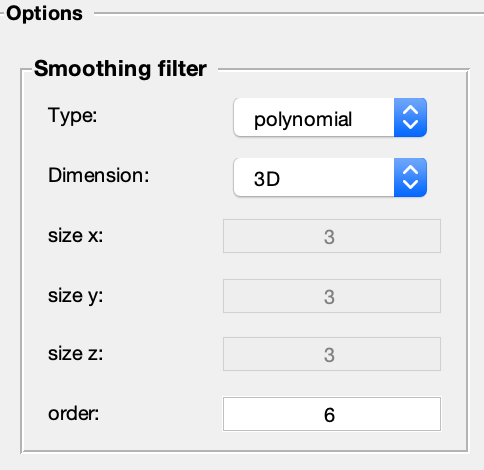
Screenshot of filtering module options in qMRLab. This new module contains a broad range of options that are customizable for the users' needs. Four filtering methods are available: Gaussian kernel, median kernel, polynomial fitting, and spline fitting. Filters can be applied in 2D or 3D mode, meaning either they are applied for single slices (in-plane) or across all three spatial directions. The size of the filters can also be customized. For Gaussian and median filters, the size (in terms of voxels) along each direction can be set. For polynomial and spline filters, the filter order can be set.
Here's an example B1 map dataset compared against the filtered output using each of the four filtering modes.
%% MATLAB/OCTAVE CODE
% Adds qMRLab to the path of the environment

cd ../qMRLab
startup
%% MATLAB/OCTAVE CODE
% Download brain MRI data

cmd = ['curl -L -o filter_map.zip https://osf.io/d8p4h/download/'];
[STATUS,MESSAGE] = unix(cmd);
unzip('filter_map.zip');
%% MATLAB/OCTAVE CODE
%

clear all

Model = filter_map;

% Format data structure so that they may be fit by the model
data = struct();
data.Raw=double(load_nii_data('Raw.nii.gz'));
data.Mask=double(load_nii_data('Mask.nii.gz'));

Model.options.Smoothingfilter_Type = 'gaussian';
filterSize = 5;
Model.options.Smoothingfilter_sizex = filterSize;
Model.options.Smoothingfilter_sizey = filterSize;
Model.options.Smoothingfilter_sizez = filterSize;
FitResults_gaussian = FitData(data,Model,0);

Model.options.Smoothingfilter_Type = 'median';
filterSize = 5;
Model.options.Smoothingfilter_sizex = filterSize;
Model.options.Smoothingfilter_sizey = filterSize;
Model.options.Smoothingfilter_sizez = filterSize;
FitResults_median = FitData(data,Model,0);

Model.options.Smoothingfilter_Type = 'polynomial';
Model.options.Smoothingfilter_order = 6;
FitResults_polynomial = FitData(data,Model,0);

Model.options.Smoothingfilter_Type = 'spline';
Model.options.Smoothingfilter_order = 2;
FitResults_spline = FitData(data,Model,0);
%% MATLAB/OCTAVE CODE
% Code used to re-orient the images to make pretty figures, and to assign variables with the axis lengths.

sliceIndex = 20;

Mask = imrotate(squeeze(data.Mask(:,:,sliceIndex)), -90);

B1map = imrotate(squeeze(data.Raw(:,:,sliceIndex)), -90).*Mask;

B1map_gaussian = imrotate(squeeze(FitResults_gaussian.Filtered(:,:,sliceIndex)), -90).*Mask;
B1map_median = imrotate(squeeze(FitResults_median.Filtered(:,:,sliceIndex)), -90).*Mask;
B1map_polynomial = imrotate(squeeze(FitResults_polynomial.Filtered(:,:,sliceIndex)), -90).*Mask;
B1map_spline = imrotate(squeeze(FitResults_spline.Filtered(:,:,sliceIndex)), -90).*Mask;

xAxis = [0:size(B1map,2)-1];
yAxis = [0:size(B1map,1)-1];
Figure 2. Raw vs Filtered B1 maps using four filters: Gaussian, median, polynomial, and spline. Gaussian filter settings: 3D filter, filter size = 5 voxels (isotropic). Median filter settings: 3D filter, filter size = 5 voxels (isotropic). Polynomial fit settings: 3D filter, filter order = 6. Spline fit settings: 3D filter, filter order = 2.
Here's a comparison of the 2D and 3D options using the Median filtering mode.
%% MATLAB/OCTAVE CODE
%

clear all

Model = filter_map;

% Format data structure so that they may be fit by the model
data = struct();
data.Raw=double(load_nii_data('Raw.nii.gz'));
data.Mask=double(load_nii_data('Mask.nii.gz'));

Model.options.Smoothingfilter_Type = 'median';
Model.options.Smoothingfilter_Dimension ='2D';
filterSize = 3;
Model.options.Smoothingfilter_sizex = filterSize;
Model.options.Smoothingfilter_sizey = filterSize;
Model.options.Smoothingfilter_sizez = filterSize;
FitResults_2D = FitData(data,Model,0);

Model.options.Smoothingfilter_Type = 'median';
Model.options.Smoothingfilter_Dimension ='3D';
filterSize = 3;
Model.options.Smoothingfilter_sizex = filterSize;
Model.options.Smoothingfilter_sizey = filterSize;
Model.options.Smoothingfilter_sizez = filterSize;
FitResults_3D = FitData(data,Model,0);
%% MATLAB/OCTAVE CODE
% Code used to re-orient the images to make pretty figures, and to assign variables with the axis lengths.

sliceIndex = 20;

Mask = imrotate(squeeze(data.Mask(60,:,:)), -90);

B1map = imrotate(squeeze(data.Raw(60,:,:)), -90).*Mask;

B1map_2D = imrotate(squeeze(FitResults_2D.Filtered(60,:,:)), -90).*Mask;
B1map_3D = imrotate(squeeze(FitResults_3D.Filtered(60,:,:)), -90).*Mask;

xAxis = [0:size(B1map,2)-1];
yAxis = [0:size(B1map,1)-1]*3;
Figure 3. A comparison between 2D and 3D median-filtered B1 maps, from a sagittal view. Median filter settings: 2D and 3D filters, filter size = 3 voxels (isotropic).
To illustrate how the filtered image is impacted by the filter order, here we show polynomial-filtered maps using three filter order values (2, 4, 6).
%% MATLAB/OCTAVE CODE
%

clear all

Model = filter_map;

% Format data structure so that they may be fit by the model
data = struct();
data.Raw=double(load_nii_data('Raw.nii.gz'));
data.Mask=double(load_nii_data('Mask.nii.gz'));


Model.options.Smoothingfilter_Type = 'polynomial';
Model.options.Smoothingfilter_Dimension ='3D';

Model.options.Smoothingfilter_order = 2;
FitResults_filterOrder_2 = FitData(data,Model,0);

Model.options.Smoothingfilter_order = 4;
FitResults_filterOrder_4 = FitData(data,Model,0);

Model.options.Smoothingfilter_order = 6;
FitResults_filterOrder_6 = FitData(data,Model,0);
%% MATLAB/OCTAVE CODE
% Code used to re-orient the images to make pretty figures, and to assign variables with the axis lengths.

sliceIndex = 20;

Mask = imrotate(squeeze(data.Mask(:,:,sliceIndex)), -90);

B1map = imrotate(squeeze(data.Raw(:,:,sliceIndex)), -90).*Mask;

B1map_filterOrder_2 = imrotate(squeeze(FitResults_filterOrder_2.Filtered(:,:,sliceIndex)), -90).*Mask;
B1map_filterOrder_4 = imrotate(squeeze(FitResults_filterOrder_4.Filtered(:,:,sliceIndex)), -90).*Mask;
B1map_filterOrder_6 = imrotate(squeeze(FitResults_filterOrder_6.Filtered(:,:,sliceIndex)), -90).*Mask;

xAxis = [0:size(B1map,2)-1];
yAxis = [0:size(B1map,1)-1];
Figure 4. Comparison of polynomial-filtered B1 maps using different of filter order values. Polynomial fit settings: 3D filter, filter order values = 2, 4, and 6.
To illustrate how the filtered image is impacted by the filter size, here we show median filtered maps using three isotropic filter sizes (1, 5, 9).
%% MATLAB/OCTAVE CODE
% Code used to generate the data required for Figure 5 of the blog post

clear all

Model = filter_map;

% Format data structure so that they may be fit by the model
data = struct();
data.Raw=double(load_nii_data('Raw.nii.gz'));
data.Mask=double(load_nii_data('Mask.nii.gz'));

Model.options.Smoothingfilter_Type = 'median';
Model.options.Smoothingfilter_Dimension ='2D';

filterSize = 1;
Model.options.Smoothingfilter_sizex = filterSize;
Model.options.Smoothingfilter_sizey = filterSize;
Model.options.Smoothingfilter_sizez = filterSize;
FitResults_filterSize_1 = FitData(data,Model,0);

filterSize = 5;
Model.options.Smoothingfilter_sizex = filterSize;
Model.options.Smoothingfilter_sizey = filterSize;
Model.options.Smoothingfilter_sizez = filterSize;
FitResults_filterSize_5 = FitData(data,Model,0);

filterSize = 9;
Model.options.Smoothingfilter_sizex = filterSize;
Model.options.Smoothingfilter_sizey = filterSize;
Model.options.Smoothingfilter_sizez = filterSize;
FitResults_filterSize_9 = FitData(data,Model,0);
%% MATLAB/OCTAVE CODE
% Code used to re-orient the images to make pretty figures, and to assign variables with the axis lengths.

sliceIndex = 20;

Mask = imrotate(squeeze(data.Mask(:,:,sliceIndex)), -90);

B1map = imrotate(squeeze(data.Raw(:,:,sliceIndex)), -90).*Mask;

B1map_filterSize_1 = imrotate(squeeze(FitResults_filterSize_1.Filtered(:,:,sliceIndex)), -90).*Mask;
B1map_filterSize_5 = imrotate(squeeze(FitResults_filterSize_5.Filtered(:,:,sliceIndex)), -90).*Mask;
B1map_filterSize_9 = imrotate(squeeze(FitResults_filterSize_9.Filtered(:,:,sliceIndex)), -90).*Mask;

xAxis = [0:size(B1map,2)-1];
yAxis = [0:size(B1map,1)-1];
Figure 5. Comparison of median-filtered B1 maps using different filter size values. Median filter settings: 2D filter, filter size values = 1, 5, and 9 voxels (isotropic).
Our user-friendly implementation of B1 filtering options in qMRLab provides the user with more tools to make an informed choice on which filter to use. For example, the filters will behave very differently in the presence of an artifact that has a single high value at a voxel, as can be seen in the example below.
%% MATLAB/OCTAVE CODE
% Code used to generate the data required for Figure 5 of the blog post

clear all

Model = filter_map;

% Format data structure so that they may be fit by the model
data = struct();
data.Raw=double(load_nii_data('Raw.nii.gz'));
data.Mask=double(load_nii_data('Mask.nii.gz'));

sliceIndex = 20;

% Create a false high value
data.Raw(46,70,sliceIndex) = 100;

Model.options.Smoothingfilter_Type = 'gaussian';
filterSize = 5
Model.options.Smoothingfilter_sizex = filterSize;
Model.options.Smoothingfilter_sizey = filterSize;
Model.options.Smoothingfilter_sizez = filterSize;
FitResults_gaussian = FitData(data,Model,0);

Model.options.Smoothingfilter_Type = 'median';
filterSize = 5
Model.options.Smoothingfilter_sizex = filterSize;
Model.options.Smoothingfilter_sizey = filterSize;
Model.options.Smoothingfilter_sizez = filterSize;
FitResults_median = FitData(data,Model,0);

Model.options.Smoothingfilter_Type = 'polynomial';
Model.options.Smoothingfilter_order = 6;
FitResults_polynomial = FitData(data,Model,0);

Model.options.Smoothingfilter_Type = 'spline';
Model.options.Smoothingfilter_order = 2;
FitResults_spline = FitData(data,Model,0);
%% MATLAB/OCTAVE CODE
% Code used to re-orient the images to make pretty figures, and to assign variables with the axis lengths.

Mask = imrotate(squeeze(data.Mask(:,:,sliceIndex)), -90);

B1map = imrotate(squeeze(data.Raw(:,:,sliceIndex)), -90).*Mask;


B1map_gaussian = imrotate(squeeze(FitResults_gaussian.Filtered(:,:,sliceIndex)), -90).*Mask;
B1map_median = imrotate(squeeze(FitResults_median.Filtered(:,:,sliceIndex)), -90).*Mask;

B1map_polynomial = imrotate(squeeze(FitResults_polynomial.Filtered(:,:,sliceIndex)), -90).*Mask;

B1map_spline = imrotate(squeeze(FitResults_spline.Filtered(:,:,sliceIndex)), -90).*Mask;

xAxis = [0:size(B1map,2)-1];
yAxis = [0:size(B1map,1)-1];
Figure 6. Impact of different filters for a simulated image artifact (high value (100) at a single voxel). Gaussian filter settings: 3D filter, filter size = 5 voxels (isotropic). Median filter settings: 3D filter, filter size = 5 voxels (isotropic). Polynomial fit settings: 3D filter, filter order = 6. Spline fit settings: 3D filter, filter order = 2.
Looking Forward
As with most open source projects, these new features will benefit from community feedback. If you encounter any bugs or have ideas for improvements, feedback is always welcome through our issues page on our GitHub repository.
We believe that a study comparing different filtering techniques for different B1 mapping techniques and types of artifacts would be very valuable to the community, as to our knowledge this hasn't been done before (reach out to us if you think it has !). If you are interested in doing such a study, we hope that qMRLab has provided you with sufficient tools to explore this further.
# PYTHON CODE

display(HTML(
    '<style type="text/css">'
    '.output_subarea {'
        'display: block;'
        'margin-left: auto;'
        'margin-right: auto;'
    '}'
    '.blog_body {'
        'line-height: 2;'
        'font-family: timesnewroman;'
        'font-size: 18px;'
        'margin-left: 0px;'
        'margin-right: 0px;'
    '}'
    '.biblio_body {'
        'line-height: 1.5;'
        'font-family: timesnewroman;'
        'font-size: 18px;'
        'margin-left: 0px;'
        'margin-right: 0px;'
    '}'
    '.note_body {'
        'line-height: 1.25;'
        'font-family: timesnewroman;'
        'font-size: 18px;'
        'margin-left: 0px;'
        'margin-right: 0px;'
        'color: #696969'
    '}'
    '.figure_caption {'
        'line-height: 1.5;'
        'font-family: timesnewroman;'
        'font-size: 16px;'
        'margin-left: 0px;'
        'margin-right: 0px'
    '</style>'
))