% **Blog post code introduction**
%
% Congrats on activating the "All cells" option in this interactive blog post =D
%
% Below, several new HTML blocks have appears prior to the figures, displaying the Octave/MATLAB code that was used to generate the figures in this blog post.
%
% If you want to reproduce the data on your own local computer, you simply need to have qMRLab installed in your Octave/MATLAB path and run the "startup.m" file, as is shown below.
%
% If you want to get under the hood and modify the code right now, you can do so in the Jupyter Notebook of this blog post hosted on MyBinder. The link to it is in the introduction above.
MP2RAGE T1 Mapping
Dictionary-based MRI techniques capable of generating T1 maps are increasing in popularity, due to their growing availability on clinical scanners, rapid scan times, and fast post-processing computation time, thus making quantitative T1 mapping accessible for clinical applications. Generally speaking, dictionary-based quantitative MRI techniques use numerical dictionaries—databases of pre-calculated signal values simulated for a wide range of tissue and protocol combinations—during the image reconstruction or post-processing stages. Popular examples of dictionary-based techniques that have been applied to T1 mapping are MR Fingerprinting (MRF) (Ma et al. 2013), certain flavours of compressed sensing (CS) (Doneva et al. 2010; Li et al. 2012), and Magnetization Prepared 2 Rapid Acquisition Gradient Echoes (MP2RAGE) (Marques et al. 2010). Dictionary-based techniques can usually be classified into one of two categories: techniques that use information redundancy from parametric data to assist in accelerated imaging (e.g. CS, MRF), or those that use dictionaries to estimate quantitative maps using the MR images after reconstruction. Because MP2RAGE is a technique implemented primarily for T1 mapping, and it is becoming increasingly available as a standard pulse sequence on many MRI systems, the remainder of this section will focus solely on this technique. However, many concepts discussed are shared by other dictionary-based techniques.
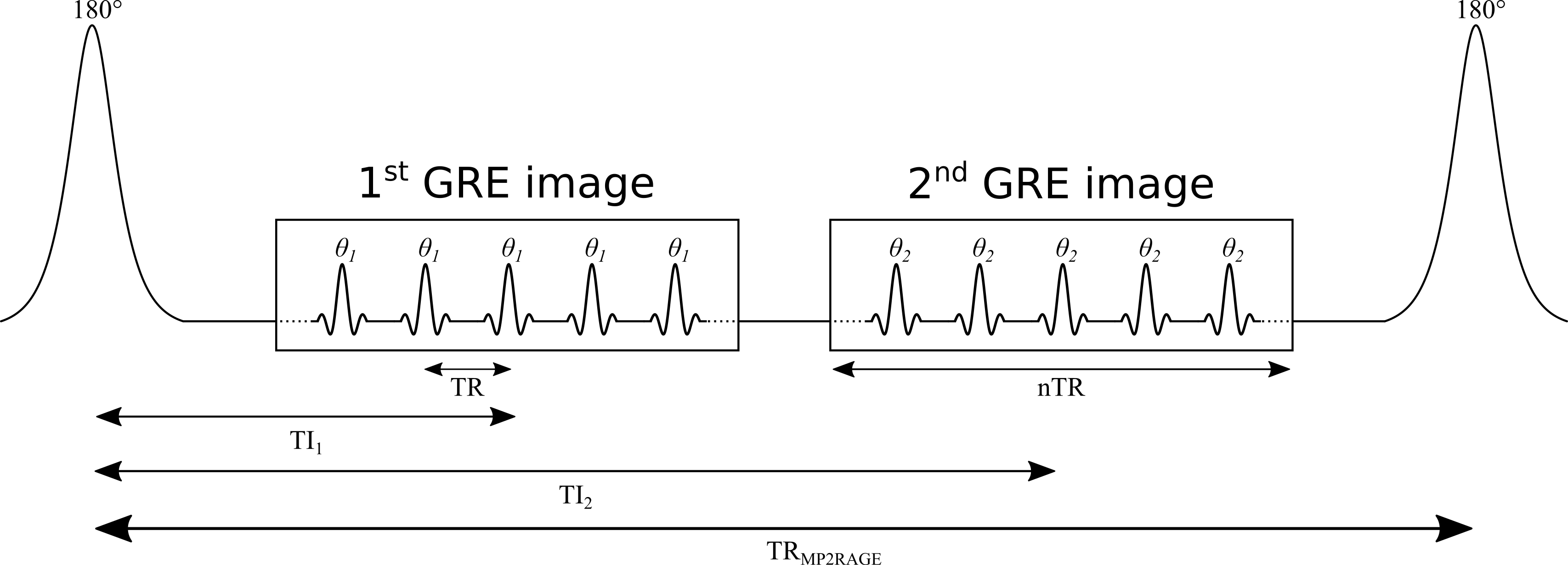
MP2RAGE is an extension of the conventional MPRAGE pulse sequence widely used in clinical studies (Haase et al. 1989; Mugler & Brookeman 1990). A simplified version of the MP2RAGE pulse sequence is shown in Figure 1. MP2RAGE can be seen as a hybrid between the inversion recovery and VFA pulse sequences: a 180° inversion pulse is used to prepare the magnetization for T1 sensitivity at the beginning of each TRMP2RAGE, and then two images are acquired at different inversion times using gradient recalled echo (GRE) imaging blocks with low flip angles and short repetition times (TR). During a given GRE imaging block, each excitation pulse is followed by a constant in-plane (“y”) phase encode weighting (varied for each TRMP2RAGE), but with different 3D (“z”) phase encoding gradients (varied at each TR). The center of k-space for the 3D phase encoding direction is acquired at the TI for each GRE imaging block. The main motivation for developing the MP2RAGE pulse sequence was to provide a metric similar to MPRAGE, but with self-bias correction of the static (B0) and receive (B1-) magnetic fields, and a first order correction of the transmit magnetic field (B1+). However, because two images at different TIs are acquired (unlike MPRAGE, which only acquires data at a single TI), information about the T1 values can also be inferred, thus making it possible to generate quantitative T1 maps using this data.
Figure 1. Simplified diagram of an MP2RAGE pulse sequence. TR: repetition time between successive gradient echo readouts, TRMP2RAGE: repetition time between successive adiabatic 180° inversion pulses, TI1 and TI2: inversion times, θ1 and θ2: excitation flip angles. The imaging readout events occur within each TR using a constant in-plane phase encode (“y”) gradient set for each TRMP2RAGE, but varying 3D phase encode (“z”) gradients between each successive TR.
Signal Modelling
Prior to considering the full signal equations, we will first introduce the equation for the MP2RAGE parameter (SMP2RAGE) that is calculated in addition to the T1 map. For complex data (magnitude and phase, or real and imaginary), the MP2RAGE signal (SMP2RAGE) is calculated from the images acquired at two TIs (SGRE,TI1 and SGRE,TI2) using the following expression (Marques et al. 2010):

This value is bounded between [-0.5, 0.5], and helps reduce some B0 inhomogeneity effects using the phase data. For real data, or magnitude data with polarity restoration, this metric is instead calculated as:

Because MP2RAGE is a hybrid of pulse sequences used for inversion recovery and VFA, the resulting signal equations are more complex. Typically, a steady state is not achieved during the short train of GRE imaging blocks, so the signal at the center of k-space for each readout (which defines the contrast weighting) will depend on the number of phase-encoding steps. For simplicity, the equations presented here assume that the 3D phase-encoding dimension is fully sampled (no partial Fourier or parallel imaging acceleration). For this case (see appendix of (Marques et al. 2010) for derivation details), the signal equations are:


where B1- is the receive field sensitivity, “eff” is the adiabatic inversion pulse efficiency, ER = exp(-TR/T1), EA = exp(-TA/T1), EB = exp(-TB/T1), EC = exp(-TC/T1). The variables TA, TB, and TC are the three different delay times (TA: time between inversion pulse and beginning of the GRE1 block, TB: time between the end of GRE1 and beginning of GRE2, TC: time between the end of GRE2 and the end of the TR). If no k-space acceleration is used (e.g. no partial Fourier or parallel imaging acceleration), then these values are TA = TI1 - (n/2)TR, TB = TI2 - (TI1 + nTR), and TC = TRMP2RAGE - (TI2 + (n/2)TR), where n is the number of voxels acquired in the 3D phase encode direction varied within each GRE block. The value mz,ss is the steady-state longitudinal magnetization prior to the inversion pulse, and is given by:


From Eqs. (3–6), it is evident that the MP2RAGE parameter SMP2RAGE (Eqs. (1.11) and (1.12)) cancels out the effects of receive field sensitivity, T2*, and M0. The signal sensitivity related to the transmit field (B1+), hidden in Eqs. (3–6) within the flip angle values θ1 and θ2, can also be reduced by careful pulse sequence protocol design (Marques et al. 2010), but not entirely eliminated (Marques & Gruetter 2013).
Data Fitting
Dictionary-based techniques such as MP2RAGE do not typically use conventional minimization algorithms (e.g. Levenberg-Marquardt) to fit signal equations to observed data. Instead, the MP2RAGE technique uses pre-calculated signal values for a wide range of parameter values (e.g. T1), and then interpolation is done within this dictionary of values to estimate the T1 value that matches the observed signal. This approach results in rapid post-processing times because the dictionaries can be simulated/generated prior to scanning and interpolating between these values is much faster than most fitting algorithms. This means that the quantitative image can be produced and displayed directly on the MRI scanner console rather than needing to be fitted offline.
Figure 2. T1 lookup table as a function of B1 and SMP2RAGE value. Inversion times used to acquire this magnitude image dataset were 800 ms and 2700 ms, the flip angles were 4° and 5° (respectively), TRMP2RAGE = 6000 ms, and TR = 6.7 ms. The code that was used were shared open sourced by the authors of the original MP2RAGE paper (https://github.com/JosePMarques/MP2RAGE-related-scripts).
%% MATLAB/OCTAVE CODE
% Code used to generate the data required for Figure 5 of the blog post

clear all
cd ../qMRLab
startup


MP2RAGE.B0=7;           % in Tesla
MP2RAGE.TR=6;           % MP2RAGE TR in seconds
MP2RAGE.TRFLASH=6.7e-3; % TR of the GRE readout
MP2RAGE.TIs=[800e-3 2700e-3];% inversion times - time between middle of refocusing pulse and excitatoin of the k-space center encoding
MP2RAGE.NZslices=[35 72];% Slices Per Slab * [PartialFourierInSlice-0.5  0.5]
MP2RAGE.FlipDegrees=[4 5];% Flip angle of the two readouts in degrees
invEFF=0.99;

B1_vector=0.005:0.05:1.9;
T1_vector=0.5:0.05:5.2;

npoints=40;


%% creates a lookup table of MP2RAGE intensities as a function of B1 and T1

k=0;
for b1val=B1_vector
    k=k+1;
    [Intensity T1vector ]=MP2RAGE_lookuptable(2,MP2RAGE.TR,MP2RAGE.TIs,b1val*MP2RAGE.FlipDegrees,MP2RAGE.NZslices,MP2RAGE.TRFLASH,'normal',invEFF);
    MP2RAGEmatrix(k,:)=interp1(T1vector,Intensity,T1_vector);
end;

%% make the matrix  MP2RAGEMatrix into T1_matrix(B1,ratio)
MP2RAGE_vector=linspace(-0.5,0.5,npoints);
k=0;
for b1val=B1_vector
    k=k+1;
    try

        T1matrix(k,:)=interp1(MP2RAGEmatrix(k,:),T1_vector,MP2RAGE_vector,'pchirp');
    catch
        temp=MP2RAGEmatrix(k,:);
        temp(isnan(temp))=linspace(-0.5,-1,length(find(isnan(temp)==1)));
        temp=interp1(temp,T1_vector,MP2RAGE_vector);

        T1matrix(k,:)=temp;

    end
end
To produce T1 maps with good accuracy and precision using dictionary-based interpolation methods, it is important that the signal curves are unique for each parameter value. MP2RAGE can produce good T1 maps by using a dictionary with only dimensions (T1, SMP2RAGE), since SMP2RAGE is unique for each T1 value for a given protocol (Marques et al. 2010). However, as was noted above, SMP2RAGE is also sensitive to B1 because of θ1 and θ2 in Eqs. (1.13–1.16). The B1-sensitivity can be reduced substantially with careful MP2RAGE protocol optimization (Marques et al. 2010), and further improved by including B1 as one of the dictionary dimensions [T1, B1, SMP2RAGE] (Figure 1.15). This requires an additional acquisition of a B1 map (Marques & Gruetter 2013), which lengthens the scan time.
Figure 3. Example MP2RAGE dataset of a healthy adult brain at 7T and T1 map. Inversion times used to acquire this magnitude image dataset were 800 ms and 2700 ms, the flip angles were 4° and 5° (respectively), TRMP2RAGE = 6000 ms, and TR = 6.7 ms. The dataset and code that was used were shared open sourced by the authors of the original MP2RAGE paper (https://github.com/JosePMarques/MP2RAGE-related-scripts).
%% MATLAB/OCTAVE CODE
% Download variable flip angle brain MRI data for Figure 7 of the blog post

cmd = ['curl -L -o mp2rage.zip https://osf.io/8x2c9/download?version=1'];
[STATUS,MESSAGE] = unix(cmd);
unzip('mp2rage.zip');
%% MATLAB/OCTAVE CODE
% Code used to generate the data required for Figure 5 of the blog post

clear all
cd ../qMRLab
startup

MP2RAGE.B0=7;           % in Tesla
MP2RAGE.TR=6;           % MP2RAGE TR in seconds
MP2RAGE.TRFLASH=6.7e-3; % TR of the GRE readout
MP2RAGE.TIs=[800e-3 2700e-3];% inversion times - time between middle of refocusing pulse and excitatoin of the k-space center encoding
MP2RAGE.NZslices=[35 72];% Slices Per Slab * [PartialFourierInSlice-0.5  0.5]
MP2RAGE.FlipDegrees=[4 5];% Flip angle of the two readouts in degrees
MP2RAGE.filenameUNI='MP2RAGE_UNI.nii'; % file with UNI
MP2RAGE.filenameINV1='MP2RAGE_INV1.nii'; % file with UNI
MP2RAGE.filenameINV2='MP2RAGE_INV2.nii'; % file with INV2

% load the MP2RAGE data - it can be either the SIEMENS one scaled from
% 0 4095 or the standard -0.5 to 0.5
MP2RAGEimg=load_untouch_nii(MP2RAGE.filenameUNI, [], [], [], [], [], []);
MP2RAGEINV1img=load_untouch_nii(MP2RAGE.filenameINV1, [], [], [], [], [], []);
MP2RAGEINV2img=load_untouch_nii(MP2RAGE.filenameINV2, [], [], [], [], [], []);

[T1map , M0map , R1map]=T1M0estimateMP2RAGE(MP2RAGEimg,MP2RAGEINV2img,MP2RAGE,0.96);

% Code used to re-orient the images to make pretty figures, and to assign variables with the axis lengths.


T1_map = imrotate(squeeze(T1map.img(:,130,:)),180);
T1_map(T1map.img>5)=0;
T1_map = T1_map*1000; % Convert to ms

xAxis = [0:size(T1_map,2)-1];
yAxis = [0:size(T1_map,1)-1];

% Raw MRI data at different TI values
S_INV1 = imrotate(squeeze(MP2RAGEINV1img.img(:,130,:)),180);
S_INV2 = imrotate(squeeze(MP2RAGEINV2img.img(:,130,:)),180);
B1map = imrotate(-0.5+1/4095*double(squeeze(MP2RAGEimg.img(:,130,:))),180);
The MP2RAGE pulse sequence is increasingly being distributed by MRI vendors, thus typically a data fitting package is also available to reconstruct the T1 maps online. Alternatively, several open source packages to create T1 maps from MP2RAGE data are available online (Marques 2017; de Hollander 2017), and for new users these are recommended—as opposed to programming one from scratch—as there are many potential pitfalls (e.g. adjusting the equations to handle partial Fourier or parallel imaging acceleration).
Benefits and Pitfalls
This widespread availability and its turnkey acquisition/fitting procedures are a main contributing factor to the growing interest for including quantitative T1 maps in clinical and neuroscience studies. T1 values measured using MP2RAGE showed high levels of reproducibility for the brain in an inter- and intra-site study at eight sites (same MRI hardware/software and at 7 T) of two subjects (Voelker et al. 2016). Not only does MP2RAGE have one of the fastest acquisition and post-processing times among quantitative T1 mapping techniques, but it can accomplish this while acquiring very high resolution T1 maps (1 mm isotropic at 3T and submillimeter at 7T, both in under 10 min (Fujimoto et al. 2014)), opening the doors to cortical studies which greatly benefit from the smaller voxel size (Waehnert et al. 2014; Beck et al. 2018; Haast et al. 2018).
Despite these benefits, MP2RAGE and similar dictionary-based techniques have certain limitations that are important to consider before deciding to incorporate them in a study. Good reproducibility of the quantitative T1 map is dependent on using one pre-calculated dictionary. If two different dictionaries are used (e.g. cross-site with different MRI vendors), the differences in the dictionary interpolations will likely result in minor differences in T1 estimates for the same data. Also, although the B1-sensitivity of the MP2RAGE T1 maps can be reduced with proper protocol optimization, it can be substantial enough that further correction using a measured B1 map should be done (Marques & Gruetter 2013; Haast et al. 2018). However B1 mapping brings an additional potential source of error, so carefully selecting a B1 mapping technique and accompanying post-processing method (e.g. filtering) should be done before integrating it in a T1 mapping protocol (Boudreau et al. 2017). Lastly, the MP2RAGE equations (and thus, dictionaries) assume monoexponential longitudinal relaxation, and this has been shown to result in suboptimal estimates of the long T1 component for a biexponential relaxation model (Rioux et al. 2016), an effect that becomes more important at higher fields.
Works Cited
Beck, E.S. et al., 2018. Improved Visualization of Cortical Lesions in Multiple Sclerosis Using 7T MP2RAGE. Am. J. Neuroradiol. Available at: http://dx.doi.org/10.3174/ajnr.A5534.
Boudreau, M. et al., 2017. B1 mapping for bias-correction in quantitative T1 imaging of the brain at 3T using standard pulse sequences. J. Magn. Reson. Imaging, 46(6), pp.1673–1682.
Doneva, M. et al., 2010. Compressed sensing reconstruction for magnetic resonance parameter mapping. Magn. Reson. Med., 64(4), pp.1114–1120.
Fujimoto, K. et al., 2014. Quantitative comparison of cortical surface reconstructions from MP2RAGE and multi-echo MPRAGE data at 3 and 7 T. NeuroImage, 90, pp.60–73.
Haase, A. et al., 1989. Inversion recovery snapshot FLASH MR imaging. J. Comput. Assist. Tomogr., 13(6), pp.1036–1040.
Haast, R.A.M., Ivanov, D. & Uludağ, K., 2018. The impact of B1+ correction on MP2RAGE cortical T1 and apparent cortical thickness at 7T. Hum. Brain Mapp., 39(6), pp.2412–2425.
de Hollander, G., 2017. PyMP2RAGE. Available at: https://github.com/Gilles86/pymp2rage [Accessed January 2, 2019].
Li, W., Griswold, M. & Yu, X., 2012. Fast cardiac T1 mapping in mice using a model-based compressed sensing method. Magn. Reson. Med., 68(4), pp.1127–1134.
Ma, D. et al., 2013. Magnetic resonance fingerprinting. Nature, 495(7440), pp.187–192.
Marques, J., 2017. MP2RAGE related scripts. Available at: https://github.com/JosePMarques/MP2RAGE-related-scripts [Accessed January 2, 2019].
Marques, J.P. et al., 2010. MP2RAGE, a self bias-field corrected sequence for improved segmentation and T1-mapping at high field. NeuroImage, 49(2), pp.1271–1281.
Marques, J.P. & Gruetter, R., 2013. New Developments and Applications of the MP2RAGE Sequence - Focusing the Contrast and High Spatial Resolution R1 Mapping. PloS one, 8(7), p.e69294.
Mugler, J.P., 3rd & Brookeman, J.R., 1990. Three-dimensional magnetization-prepared rapid gradient-echo imaging (3D MP RAGE). Magn. Reson. Med., 15(1), pp.152–157.
Rioux, J.A., Levesque, I.R. & Rutt, B.K., 2016. Biexponential longitudinal relaxation in white matter: Characterization and impact on T1 mapping with IR-FSE and MP2RAGE. Magn. Reson. Med., 75(6), pp.2265–2277.
Voelker, M.N. et al., 2016. The traveling heads: multicenter brain imaging at 7 Tesla. Magma, 29(3), pp.399–415.
Waehnert, M.D. et al., 2014. Anatomically motivated modeling of cortical laminae. NeuroImage, 93 Pt 2, pp.210–220.
Errata
A previous version of this text incorrectly stated the equations for TB and TC. They were written as TB = TI2 - TI1 + (n/2)TR and TC = TRMP2RAGE - TI2 + (n/2)TR, whereas they should have been TB = TI2 - (TI1 + nTR) and TC = TRMP2RAGE - (TI2 + (n/2)TR). This has been corrected in the text. Thank you to Marc-Antoine Fortin (LinkedIn, Twitter) from the MRI Methods Research Group at McGill University for notifying us of this error.
# PYTHON CODE

display(HTML(
    '<style type="text/css">'
    '.output_subarea {'
        'display: block;'
        'margin-left: auto;'
        'margin-right: auto;'
    '}'
    '.blog_body {'
        'line-height: 2;'
        'font-family: timesnewroman;'
        'font-size: 18px;'
        'margin-left: 0px;'
        'margin-right: 0px;'
    '}'
    '.biblio_body {'
        'line-height: 1.5;'
        'font-family: timesnewroman;'
        'font-size: 18px;'
        'margin-left: 0px;'
        'margin-right: 0px;'
    '}'
    '.note_body {'
        'line-height: 1.25;'
        'font-family: timesnewroman;'
        'font-size: 18px;'
        'margin-left: 0px;'
        'margin-right: 0px;'
        'color: #696969'
    '}'
    '.figure_caption {'
        'line-height: 1.5;'
        'font-family: timesnewroman;'
        'font-size: 16px;'
        'margin-left: 0px;'
        'margin-right: 0px'
    '</style>'
))